
Every real dataset arrives with two problems before you write a line of modelling code. Some values are missing. Other values are technically present but look wrong. How you handle them decides more about your model than most hyperparameter searches will.
The good news is that neither problem needs a clever trick. It needs a short sequence of questions, asked in the right order: what is missing or extreme, why, and what does the model need? This guide works through both problems on one dataset, with the code for each step and the numbers it actually produces.
The dataset
I'll use the Titanic passenger list that ships with seaborn. It is small enough to reason about, and it contains every kind of mess this guide covers:
- a column that is mostly empty
- a column with a meaningful gap
- two stray blanks
- a fare column with a very long tail
import numpy as np
import pandas as pd
import seaborn as sns

df = sns.load_dataset("titanic")
df.shape(891, 15)Everything below runs on pandas 3.1 and scikit-learn 1.9, but none of it depends on recent features.
Part 1: Missing values
Find them first
Before deciding anything, measure. Counts alone are misleading on a large table, so put the percentage next to each one.
missing = (
    df.isna().sum().to_frame("missing")
    .assign(percent=lambda t: (t["missing"] / len(df) * 100).round(1))
    .query("missing > 0")
    .sort_values("missing", ascending=False)
)
missing missing percent
deck 688 77.2
age 177 19.9
embarked 2 0.2
embark_town 2 0.2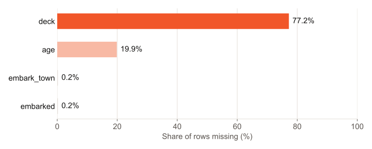
Those four columns look like one problem. They are three, and each gets a different answer.
Ask why it is missing
The method you choose depends on why a value is absent. Statisticians sort missingness into three kinds, and the names are worth knowing because they map directly to decisions:
- Missing completely at random (MCAR): the gap has nothing to do with anything. A sensor dropped a packet. Dropping those rows loses data, but doesn't bias what's left.
- Missing at random (MAR): the gap depends on other columns you have. You can model around it, because the explanation is in the data.
- Missing not at random (MNAR): the gap depends on the missing value itself. People with high incomes skip the income question. No imputation (filling in the gaps) fixes this cleanly. The missingness is information.
You can't prove which kind you have, but you can look for evidence. Check whether the gap moves with other columns:
df["deck"].isna().groupby(df["pclass"]).mean().round(3)pclass
1 0.190
2 0.913
3 0.976The deck is missing for 19% of first-class passengers and 98% of third-class ones. That is not random. The gap tracks ticket class. Filling it with "the most common deck" would invent cabins for people who almost certainly didn't have one on record.
Age shows a milder version of the same pattern:
df["age"].isna().groupby(df["pclass"]).mean().round(3)pclass
1 0.139
2 0.060
3 0.277df.groupby(df["age"].isna())["survived"].mean().round(3)age
False 0.406
True 0.294Passengers with no recorded age survived at 29%, against 41% for everyone else. Whatever caused the gap moves with the outcome you would predict. Keep that in mind. It comes back below.
Option 1: Drop it
Dropping data is the right call more often than people admit, but only at the right grain.
len(df.dropna())                  # 182 rows survive, out of 891
len(df.dropna(subset=["age"]))    # 714
A blanket dropna() removes 80% of the data because of one column. Drop the column when it is mostly empty and you can't recover its meaning (here, deck). Drop rows only when the gap affects very few of them and looks random. The two missing embarked values qualify: two rows out of 891 is noise, whatever you do with them.
df = df.drop(columns=["deck"])Option 2: Fill with a simple statistic
For a numeric column, the median is the safe default. Extreme values do not distort it, and it is always a value the column could plausibly hold. For a categorical column, use the most frequent value.
print(f"skew {df['age'].skew():.2f}, mean {df['age'].mean():.1f}, median {df['age'].median():.1f}")skew 0.39, mean 29.7, median 28.0Age is only slightly skewed, so the mean and median are close here. On a column like income, they can be miles apart. With scikit-learn, the same thing is a SimpleImputer:
from sklearn.impute import SimpleImputer

SimpleImputer(strategy="median")          # numeric columns
SimpleImputer(strategy="most_frequent")   # categorical columns
The cost of a single statistic is that every filled row gets the same value. Fill 177 ages with 28, and you create a spike at 28 and shrink the column's variance.
Option 3: Fill within groups
You can do much better by filling from rows that resemble the missing one. Age varies a lot by class and sex, so a 3rd-class woman and a 1st-class man shouldn't receive the same guess:
df.groupby(["pclass", "sex"])["age"].median()pclass sex
1 female 35.0
male 40.0
2 female 28.0
male 30.0
3 female 21.5
male 25.0age_filled = df["age"].fillna(
df.groupby(["pclass", "sex"])["age"].transform("median")
)transform returns a value for every row, aligned to the original index, which is what makes it a one-line fill. The guesses now range from 21.5 to 40 instead of sitting on a single number.
Option 4: Let a model fill it
When several columns predict the missing one, a model can use all of them at once. scikit-learn ships two:
from sklearn.experimental import enable_iterative_imputer  # noqa: F401
from sklearn.impute import IterativeImputer, KNNImputer

cols = ["age", "fare", "pclass", "sibsp", "parch"]
KNNImputer(n_neighbors=5).fit_transform(df[cols])
IterativeImputer(random_state=0).fit_transform(df[cols])
KNNImputer averages the five most similar passengers. IterativeImputer fits a regression for each column against the others and repeats until the estimates settle. On this data, the imputed ages average 30.5 (KNN) and 27.7 (iterative). Both are close to the median, but they now vary with each passenger's fare and family size. These are worth the extra complexity when the relationships are strong. When they aren't, they mostly add runtime.
Keep the signal: flag what you filled
Remember that missing ages survived at a different rate. If you fill the gap and continue, the model can no longer see that a value was ever missing. Add an indicator column, so it can:
imputer = SimpleImputer(strategy="median", add_indicator=True)
imputer.fit(df[["age"]]).get_feature_names_out()['age', 'missingindicator_age']This is the most underused option in the toolkit. It costs one column, and a model that doesn't need it can learn to ignore it. It is also the honest answer to data that might be missing not at random.
The leakage trap
Every example above computed its statistic on the whole dataset. In a notebook that's harmless. In a model, it's a leak. The median that fills the test set comes partly from the test set. So your evaluation sees data it should never see. On a small or shifting dataset, that is enough to make a model look better than it will perform.
The fix is structural, not a matter of being careful. Put the imputer inside a Pipeline, so it learns its statistics from the training fold only, every time:
from sklearn.compose import ColumnTransformer
from sklearn.linear_model import LogisticRegression
from sklearn.model_selection import cross_val_score, train_test_split
from sklearn.pipeline import Pipeline, make_pipeline
from sklearn.preprocessing import OneHotEncoder, StandardScaler

df = sns.load_dataset("titanic")
X = df[["pclass", "sex", "age", "sibsp", "parch", "fare", "embarked"]]
y = df["survived"]
X_train, X_test, y_train, y_test = train_test_split(
    X, y, test_size=0.2, stratify=y, random_state=42
)

preprocess = ColumnTransformer([
    ("num", make_pipeline(
        SimpleImputer(strategy="median", add_indicator=True),
        StandardScaler(),
    ), ["age", "sibsp", "parch", "fare"]),
    ("cat", make_pipeline(
        SimpleImputer(strategy="most_frequent"),
        OneHotEncoder(handle_unknown="ignore"),
    ), ["pclass", "sex", "embarked"]),
])

model = Pipeline([
    ("prep", preprocess),
    ("clf", LogisticRegression(max_iter=1000)),
])

cross_val_score(model, X_train, y_train, cv=5).mean()   # 0.796
model.fit(X_train, y_train).score(X_test, y_test)        # 0.810
After fitting, the imputer's learned median age is 28.5, not the 28.0 of the full dataset. That half-year is the leak, made visible. It is small here, but not on every dataset. With a pipeline, cross_val_score refits the imputer inside each fold automatically. In production, the same object fills new data with exactly the statistics it learned in training.
Part 2: Outliers
Look before you remove anything
An outlier is a value far from the rest. That's all the word means. It does not mean "wrong", and the most common mistake in this whole topic is treating the two as the same thing.
df["fare"].describe().round(2)count 891.00
mean 32.20
std 49.69
min 0.00
25% 7.91
50% 14.45
75% 31.00
max 512.33The mean is more than double the median. The maximum is more than sixteen times the upper quartile. The skew is 4.79, where a symmetric column sits near 0. This column has a long right tail. The question is what's in it.
df.nlargest(4, "fare")[["fare", "pclass", "embark_town", "alive"]] fare pclass embark_town alive
258 512.3292 1 Cherbourg yes
679 512.3292 1 Cherbourg yes
737 512.3292 1 Cherbourg yes
27 263.0000 1 Southampton noThree first-class passengers paid exactly the same top fare, boarded at the same port, and all survived. That is a booking, not a typo. Dropping those rows would lose real, informative passengers. There are also 15 fares of exactly zero, which is a more interesting question: crew, or a data-entry default? A spike at 0 deserves a look before any rule touches it.
The IQR rule
The interquartile range (IQR) is the spread of the middle half of the data. The rule flags anything more than 1.5 × IQR beyond the quartiles. It is what a box plot's whiskers draw.
q1, q3 = df["fare"].quantile([0.25, 0.75])
iqr = q3 - q1
lower, upper = q1 - 1.5 * iqr, q3 + 1.5 * iqr
outliers = df[(df["fare"] < lower) | (df["fare"] > upper)]

print(f"q1 {q1:.2f}, q3 {q3:.2f}, iqr {iqr:.2f}")
print(f"lower {lower:.2f}, upper {upper:.2f}")
print(f"{len(outliers)} flagged ({len(outliers) / len(df):.1%} of passengers)")q1 7.91, q3 31.00, iqr 23.09
lower -26.72, upper 65.63
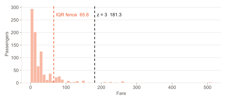
116 flagged (13.0% of passengers)Two things stand out. The lower fence is negative, so on a column that can't go below zero, the rule can only ever flag the top. And 104 of the 116 flagged fares are first-class. The rule found no errors. It found the first-class cabin.
The z-score rule
The z-score measures distance from the mean in standard deviations, and |z| > 3 is the usual cut-off:
z = (df["fare"] - df["fare"].mean()) / df["fare"].std()
(z.abs() > 3).sum()20Only 20, and the lowest flagged fare is 211.34. The z-score assumes a roughly symmetric, bell-shaped column, and fare is neither. The extreme values inflate the very standard deviation that judges them. So the cut-off lands at 181.3, and most of the tail hides under it.
For skewed data, there is a variant that resists outliers: the modified z-score. It uses the median and the median absolute deviation (MAD) instead of the mean and standard deviation:
med = df["fare"].median()
mad = (df["fare"] - med).abs().median()
modified_z = 0.6745 * (df["fare"] - med) / mad
(modified_z.abs() > 3.5).sum()160It flags 160, more than the IQR rule. The reason is that half of all fares sit within 6.90 of the median. By that yardstick, the tail is enormous. Three methods, three answers: 20, 116, 160. That's the real lesson. An outlier rule is a definition you choose, not a fact you discover, so choose it knowing what the column looks like.
Several columns at once
Single-column rules miss rows that are unusual only in combination: a young passenger travelling alone on a family-sized fare, for instance. IsolationForest scores each row by how easy it is to isolate from the rest:
from sklearn.ensemble import IsolationForest

cols = ["age", "fare", "sibsp", "parch"]
X = df[cols].fillna(df[cols].median())
iso = IsolationForest(contamination=0.02, random_state=42).fit(X)
flagged = df[iso.predict(X) == -1]
With contamination=0.02 it flags 18 rows, among them the three top fares and a cluster of 263 fares belonging to large families travelling together. Note that contamination is you deciding that 2% of the data is anomalous. It's a dial, not a measurement.
What to do with them
Once you know what an outlier is, there are four honest options:
| Situation | What to do | On this data |
|---|---|---|
| It's an error (impossible value, unit mix-up) | Fix it if you can, otherwise remove it | Check the 15 zero fares first |
| It's real, and the model is sensitive to scale | Transform the column | np.log1p takes skew from 4.79 to 0.39 |
| It's real, but too extreme to learn from | Cap it at a fence | Capping at 65.63 takes skew to 1.08 |
| It's real and it matters | Keep it, and use a model that copes | Tree models split on order, not distance |
df["fare_log"] = np.log1p(df["fare"])                 # skew 0.39
df["fare_capped"] = df["fare"].clip(upper=upper)      # skew 1.08
A log transform is usually the best first move for a money-like column. It keeps every row and every ordering, and only compresses the distances. The code uses log1p rather than log because log1p handles the zero fares. Capping is blunter: every fare above 65.63 becomes 65.63, so a 70 and a 512 become indistinguishable. Winsorizing (clipping at the 1st and 99th percentiles) is gentler still, and it barely helps here (skew 3.11). The problem is the whole tail, not the top 1%.
Whatever you choose, the leakage rule from Part 1 applies again. Fences, percentiles and means are statistics, so compute them on training data only, inside the pipeline.
A checklist
- Measure what's missing, as a percentage, and look at what's extreme before touching anything.
- Ask why. Check whether gaps and extremes move with other columns. That decides everything after.
- Drop columns that are mostly empty and unrecoverable. Drop rows only when they're few and the gap looks random.
- Impute with the median, a group median, or a model, and add an indicator whenever missingness might carry signal.
- Treat outliers as data until proven otherwise. Transform before you cap, and cap before you drop.
- Fit every statistic inside a pipeline, so nothing about the test set leaks into training.
None of this is glamorous. But a model is only ever as honest as the data you train it on. These two steps are where you win or lose that honesty.